
일반화와 과대적합
학습 데이터와 새 데이터의 RMSE를 비교하여 결정나무의 일반화와 과대적합을 이해
학습한 자료와 새로운 자료
- 일반화(generalization): 학습한 패턴을 새로운 사례에도 적용하는 능력
- 과대적합(overfitting): 학습 데이터에는 지나치게 잘 맞지만 새로운 데이터에서는 성능이 낮아지는 현상
좋은 모형은 학습 데이터를 그대로 외우는 모형이 아니라 새로운 사례도 잘 예측하는 모형.
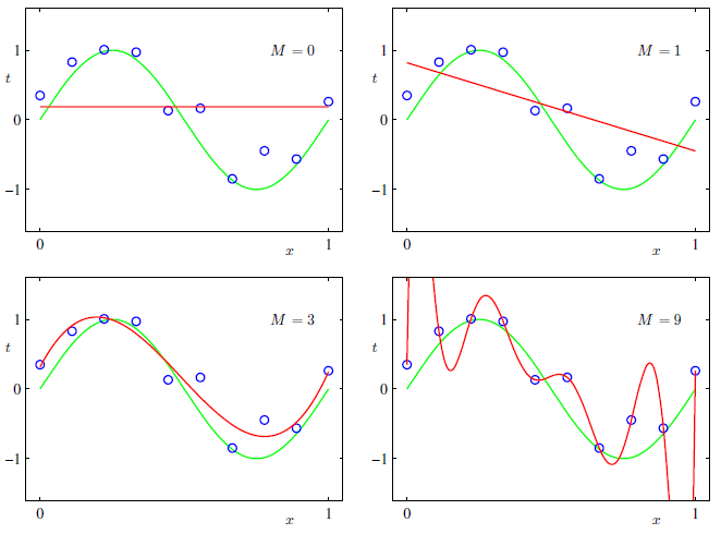
- 그림 설명:
- 녹색 곡선: 데이터가 따르는 실제 패턴(사인 함수)
- 파란 원: 학습 데이터
- 빨간 곡선: 다항식 모형의 예측
- M=0: 0차 함수. 평균만으로 예측.
- M=1: 1차 함수. 너무 단순하여 실제 패턴과 거리가 있음.
- M=3: 3차 함수. 실제 패턴과는 다른 함수지만 대체로 비슷한 패턴.
- M=9: 9차 함수. 학습한 데이터에 대해서는 오차 없이 맞추지만, 실제 패턴과는 거리가 멀어짐.
실습 준비
다운로드 명령
!wget -q -O reaction_time.xlsx "https://www.mindscale.kr/content-assets/24d730234f8d72bad3fb2f2ff9916b717797f485510adf57d80e556596de27d1/reaction_time.xlsx"
import pandas as pd
from sklearn.metrics import root_mean_squared_error
from sklearn.tree import DecisionTreeRegressor

df = pd.read_excel("reaction_time.xlsx", sheet_name="data")
학습 데이터와 새 데이터 준비
처음 120개 사례는 모형 학습에 사용하고, 나머지 200개 사례는 모형이 처음 보는 새 데이터로 남김. 반응시간에는 연습 시간에 따른 경향과 무작위 개인차가 함께 포함됨.
train_df = df.iloc[:120]
new_df = df.iloc[120:]

X_train = train_df.drop(columns="reaction_time_ms")
y_train = train_df["reaction_time_ms"]
X_new = new_df.drop(columns="reaction_time_ms")
y_new = new_df["reaction_time_ms"]
깊이 3 나무
tree3 = DecisionTreeRegressor(
    max_depth=3, random_state=42
)
tree3.fit(X_train, y_train)

pred_train3 = tree3.predict(X_train)
pred_new3 = tree3.predict(X_new)
학습 데이터의 RMSE:
root_mean_squared_error(y_train, pred_train3)
실행 결과
28.473862595618645
새 데이터의 RMSE:
root_mean_squared_error(y_new, pred_new3)
실행 결과
31.43572816272745
깊이 제한 없는 나무
tree_unlim = DecisionTreeRegressor(random_state=42)
tree_unlim.fit(X_train, y_train)

pred_train_unlim = tree_unlim.predict(X_train)
pred_new_unlim = tree_unlim.predict(X_new)
학습 데이터의 RMSE:
root_mean_squared_error(y_train, pred_train_unlim)
실행 결과
0.0
새 데이터의 RMSE:
root_mean_squared_error(y_new, pred_new_unlim)
실행 결과
42.64891244247852
학습 성능과 일반화 성능
- 학습 데이터: 깊이 제한 없는 나무의 RMSE가 0이므로 더 좋은 결과
- 새 데이터: 깊이 3 나무의 RMSE가 약 31.4ms로 제한 없는 나무의 42.6ms보다 작음
- 과대적합: 제한 없는 나무가 학습 사례의 무작위 개인차까지 외워 새 데이터의 오차가 커진 상태
모형 선택에서는 학습 데이터의 가장 작은 오차보다 새 데이터의 오차가 더 중요.
나무 깊이에 따른 예측 오차
깊이 1부터 제한 없는 나무의 실제 깊이까지 바꾸며 학습 데이터와 새 데이터의 RMSE를 비교.
import matplotlib.pyplot as plt

depths = list(range(1, tree_unlim.get_depth() + 1))
train_rmse = []
new_rmse = []
for depth in depths:
    tree = DecisionTreeRegressor(max_depth=depth, random_state=42)
    tree.fit(X_train, y_train)
    train_rmse.append(root_mean_squared_error(y_train, tree.predict(X_train)))
    new_rmse.append(root_mean_squared_error(y_new, tree.predict(X_new)))

fig, ax = plt.subplots(figsize=(7, 4))
ax.plot(depths, train_rmse, "o-", label="Train")
ax.plot(depths, new_rmse, "o-", label="Test (new data)")
ax.set_xlabel("Tree depth")
ax.set_ylabel("RMSE (ms)")
ax.set_xticks(depths)
ax.grid(alpha=0.25)
ax.legend()
fig.tight_layout()
plt.show()
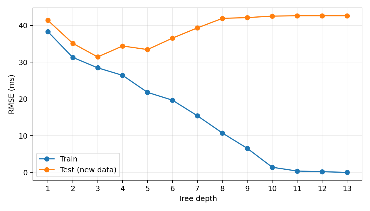
- 학습 RMSE: 깊이가 커질수록 감소하여 깊이 13에서 0ms
- 새 데이터 RMSE: 깊이 3에서 약 31.4ms로 가장 작고, 깊이 13에서는 약 42.6ms
- 학습 오차가 줄어도 새 데이터의 오차가 함께 줄지는 않음
퀴즈
일반화를 잘하는 모형은 어떤 모형인가요?
퀴즈를 풀려면 대화형 기능을 불러와야 합니다.